Synthetic trees, plots and scans

sylva.synthetic makes point clouds whose right answer is known, so that a method can be checked against the truth rather than against another method. It has two levels.

• Simple scenes (tree, forest, stand, crown_forest, scan, als_flight, forest_epochs): straight cylinder stems with a few limbs and loose leaf discs, and a scan that takes the nearest point in each angular cell. They are small and fast, the tests and examples are built on them, and their output does not change.
• Realistic scenes (tree_model, plot, and scan with a finite beam): trees with recursive branching, allometric sizes and pipe-model radii, leaves of known size and orientation, mixed stands on rough terrain with understorey and dead wood, and a scanner with range noise, a beam footprint, mixed pixels and multiple returns. Every generated object comes with its truth.

A tree and its truth

import numpy as np
from sylva import synthetic

t = synthetic.tree_model("eucalypt", dbh=0.5, height=30, epicormic=4, seed=1)
t.dbh, t.height                  # 0.5, 29.4  (m; area-equivalent DBH at 1.3 m)
t.wood_volume, t.leaf_area       # 1.867 m³, 135.6 m² (epicormic: 4.2 m²)
t.volume_by_order()              # {0: 1.747, 1: 0.071, 2: 0.035, 3: 0.014}
t.qsm                            # the wood as cylinders: a sylva.qsm.QSM
t.leaves["normal"], t.leaves["area"]
t.leaf_angles().mean_deg         # 63.3 (erectophile: 63.2)
t.leaf_angles().g(np.radians([0, 45, 90]))   # G function: 0.43, 0.48, 0.54
t.points.attrs["label"]          # 2 stem, 3 branch, 4 leaf

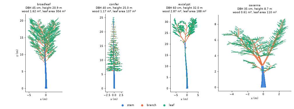
A tree is grown from an archetype:

archetype	form	leaves
broadleaf	crown from 35 % of the height, ellipsoidal; the stem forks into two limbs at 80 %	planophile, 10 × 5 cm
conifer	central leader to the top, whorls of five drooping branches from 25 %, conical crown	spherical, 5 × 1.2 cm blades standing in for shoots
eucalypt	clear bole to 55 %, three ascending limbs from 65 %, sparse crown, noticeable lean	erectophile (pendulous), 15 × 3 cm
savanna	short bole forking at 30 % into three spreading limbs, wide flat crown	planophile, 4 × 1.5 cm
shrub	several stems from near the ground (used for the understorey of plot)	spherical, 5 × 2.5 cm

synthetic.archetype(name) lists the constants behind each.

Stem. The axis leans (lean, degrees) and curves smoothly (three sinusoids per horizontal component, slope amplitude sweep). Below the lowest branch the radius follows r(s) = R g(s) / g(1.3) along the stem, with g(s) = (1 + b exp(-s / 0.6)) ((S - s) / (S - 1.3))^p: a taper of exponent p over the stem length S with butt swell b, so the diameter at 1.3 m is dbh exactly. Options give an elliptical section (ellipticity), bark fissures (bark_depth, m), both rescaled to keep the area of the round section, and buttress flanges (buttresses, buttress_height, buttress_extent), which add area.

Branches. First-order branches leave the stem from the crown base up, in whorls for the conifer and spirally at 137.5 degrees otherwise, with a length set by the archetype's crown envelope at their height; forking archetypes end the stem in codominant limbs. Each axis carries children up to max_order (1 to 4), each a fixed fraction of its parent's length and shorter towards its tip, at the archetype's branching angle, alternately to either side; axes bend upwards or droop by a tropism per metre.

Radii: the pipe model. Above the lowest branch every segment's cross-sectional area is proportional to the leaf area it carries (Shinozaki et al. 1964), r = c W^(1/e) with e = pipe_exponent (2 for the pipe model), c set so that the radius is continuous with the stem taper where the crown begins. Area is therefore conserved at every fork.

Leaves are planar elliptical blades of known length and width (area π L W / 4) on the distal 80 % of the terminal twigs. Their number is set by the leaf area, leaf_area or by default min(lai π R², leaf_k dbh²) from the archetype, and their normals are drawn from the leaf angle distribution lad: a de Wit (1965) name (spherical, planophile, erectophile, plagiophile, extremophile, uniform), ("beta", mu, nu) with Goel and Strebel's (1984) parameters, or ("ellipsoidal", chi) (Campbell 1990), uniform in azimuth.

Epicormic shoots (epicormic, shoots per metre of bole) are short leafy shoots along the bole below the crown, as on eucalypts resprouting after fire (Tumbarumba). They are flagged in the epicormic attribute and in leaves["epicormic"], so their effect on a QSM (see stem_radius_cap in QSMs) or on leaf area can be measured.

Points are drawn at point_density per m² on a jittered grid (one random point in each cell of a nearly square grid) on the wood surface and on one side of each leaf, and carry their surface normal (normal_x, normal_y, normal_z). The wood points lie exactly on the cylinders of t.qsm (on the shaped section for the stem, whose table radius is the area-equivalent one), so the table's volume is the volume of the sampled surface, and n_points counts the points on each cylinder.

The truth

truth	where
wood volume, per order, lengths	t.qsm (total_volume, stem_volume, ...), t.volume_by_order(), t.length_by_order()
leaf area and each leaf	t.leaf_area, t.epicormic_leaf_area, t.leaves (centre, normal, axis, length, width, area, cylinder)
leaf angle distribution and G	t.leaf_angles() (area-weighted), its .g(zenith)
DBH, stem position at breast height	t.dbh, t.stem_bh (a leaning stem is found there, not above its base)
height, crown	t.height, t.crown_base, t.crown_area (convex hull from above), t.crown_extent
per point	classification (4 leaf, 5 wood), label, branch_order, cylinder, leaf, epicormic

A plot

p = synthetic.plot(size=30, density=600, dbh=("weibull", 1.8, 0.22),
                   archetypes={"broadleaf": 1, "eucalypt": 1, "conifer": 1},
                   slope=0.15, roughness=0.08, seed=1)
p.stem_density, p.basal_area     # 600 stems/ha, 27.6 m²/ha
p.trees["dbh"], p.trees["height"], p.trees["wood_volume"], p.trees["leaf_area"]
p.qsm(1)                         # the cylinders of tree 1
p.ground_height(x, y)            # the terrain
p.points.attrs["label"]          # 1 ground, 2 stem, 3 branch, 4 leaf, 5 understorey, 6 dead wood

round(density * size² / 10⁴) diameters are drawn from a Weibull (("weibull", shape, scale)) or reverse-J (("reverse_j", mean), a negative exponential above min_dbh, de Liocourt's constant quotient) distribution, or given as a list. Each tree takes an archetype by weight and a height from the archetype's Chapman-Richards curve 1.3 + a (1 - exp(-b D))^c (D in cm; Richards 1959) with lognormal scatter height_noise. Stems are placed at random, largest first, never closer than 0.75 (D_i + D_j) + 0.2 m, so no two overlap at the base. The terrain is a plane rising by slope per metre towards aspect plus a Gaussian random field of standard deviation roughness and correlation length roughness_length. Understorey shrubs, grass tufts, fallen logs and stumps are scattered over the plot (shrubs, grass_cover, logs, stumps), and nothing is drawn below the ground. The trees are grown in parallel, each with its own seed, so a seed gives the same plot on any number of threads.

p.trees is the truth table: tree id, archetype, base position, the stem position at breast height (x_bh, y_bh), DBH, height above the terrain, crown base and area, wood, stem and branch volume, and leaf area. The cylinders, leaves (with their tree) and dead wood are tables too.

A scan with a finite beam

Giving scan any beam option switches from the point-cell scan to a scanner with a finite beam, cast into the points:

s = synthetic.scan(p.points, origin=(15, 15, 1.5 + p.ground_height(15, 15)),
                   resolution_deg=0.06, scanner="vz400", range_noise=0.005, seed=1)
s.echo_attrs["label"]            # the truth survives into the echoes
s.echo_attrs["range_spread"]     # m; large for a mixed pixel
s.echo_attrs["reflectance"]      # dB; 0 dB is a white target filling the footprint

• Pattern. Pulses leave on a regular zenith / azimuth grid of step resolution_deg, from min_zenith_deg to max_zenith_deg. A scanner model ("vz400", "vz400i", "vz2000i") sets the field of view (+60 to -40 degrees), beam divergence (0.35 or 0.27 mrad), exit diameter and ranging precision from the data sheets (synthetic.scanner_preset); explicit options override it. Every pulse is kept, misses included, so the shots are valid input to ray tracing.
• Footprint. A pulse is a cone of full divergence beam_divergence (mrad) from an aperture of exit_diameter, sampled by footprint_samples equal-energy sub-beams on a sunflower pattern (Vogel 1979). Each point stands for a small patch of surface of radius target_radius (by default 1.75 times the median point spacing): a disc facing along the point's normal, or a sphere where no normal is known. Discs seen edge-on are not hit, so silhouettes stay sharp.
• Echoes. Hits closer in range than echo_separation (the receiver's range resolution) form one echo; with mixed_pixels its range is the energy-weighted mean of the hits' ranges (energy: the sub-beam's share times the target's reflectance). A footprint that straddles an edge thus puts a point in the gap between foreground and background, as real mixed pixels do; hits farther apart give separate returns (multiple returns within a footprint). Echoes below detection_threshold are lost and at most max_echoes are kept, nearest first.
• Noise. Gaussian range noise of standard deviation range_noise, or a + b R for range_noise=(a, b), is added along the beam.

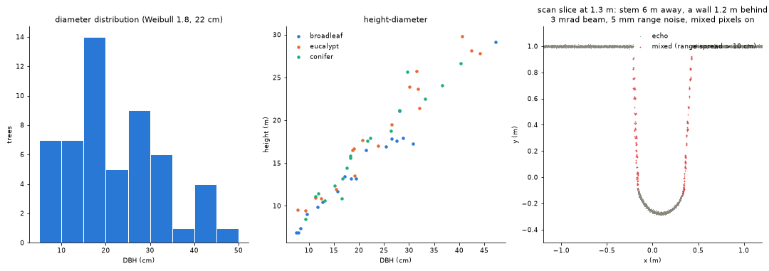
The right panel scans a stem 6 m away with a wall 1.2 m behind it, with a 3 mrad beam (wider than any real scanner's, to make the effect visible), 5 mm range noise and mixed pixels on: the red echoes, whose hits spread over more than 10 cm in range, trail from the stem's edges towards the wall.

Checks against the truth

The test suite (tests/test_synthetic_model.py) checks that:

• wood and leaf points lie on their cylinders and blades, the cylinder table gives the volume per order and in total, the leaf table gives the leaf area, and area is conserved at every fork;
• a bare stem is the analytic cone of its taper to 1 %;
• the leaf inclinations follow the requested distribution (mean against the analytic mean, a Kolmogorov-Smirnov test for the beta case) and the G function of the generated leaves matches the textbook distribution's to 0.01; azimuths are uniform;
• a plot has the requested number of stems, its diameters follow the truncated Weibull or reverse-J distribution (Kolmogorov-Smirnov), heights follow the allometry, stems do not overlap, and the terrain has the requested slope and roughness;
• the scanner's range noise has the requested standard deviation (constant and range-dependent), the number of mixed pixels at an edge follows the footprint size and angular step, none appear without mixing or with a finer range resolution (two returns instead), and the reflectance of a target filling the footprint is its own;
• a seed gives the same tree, plot and scan, and the simple scenes are unchanged (the parity recordings pass).

Sylva's own tools on a 30 × 30 m plot of 54 trees (broadleaf, eucalypt, conifer) scanned from five positions with the VZ-400 model at 0.06 degrees and 5 mm noise: trees.detect_stems found all 54 stems, with a DBH bias of +0.5 cm and an RMSE of 0.6 cm; leaves.classify_leaf_wood reached 0.91 to 0.97 accuracy on the three largest trees; qsm.build_qsm on the true wood echoes recovered 51 to 97 % of the four largest trees' wood volume, mostly the stem, as the scans see little of the crowns' small branches.

Limitations

• The trees are architectural models, not grown ones: branch angles and lengths follow fixed rules with random scatter; there is no competition between crowns, no dead branches, and conifer needles are small planar blades standing in for shoots.
• The scanner casts beams into points, not surfaces. A point stands for a patch of radius target_radius, so anything thinner than that radius (twigs, grass, leaf edges) is seen thicker than it is, and a surface sampled with independent random points rather than a jittered grid lets a few sub-beams through. The default radius is set from the median spacing over the whole scene; where densities differ a lot, give target_radius.
• Range noise is Gaussian; there is no intensity-dependent ranging bias, no atmospheric attenuation and no waveform shape (see Full waveforms for those).